Documentation of GWXtreme

Introduction:

GWXtreme package hosts tools for inferences on extreme matter using gravitational wave parameter estimation data. Currently available tools include the following:

1. Model selection of the neutron star equation of state using gravitational wave parameter estimation results.

Neutron star equation of state model selection:

Our knowledge of the equation of state of neutron star exhibits a fundamental gap in our understanding of matter at extreme density and pressure. It is impossible to replicate such environments in human-made laboratories, making us relying entirely on astrophysical observations. Investigations conducted in this field have been predominantly focussed on observation of pulsars and x-ray binaries in the electromagnetic spectrum.

The direct detection and characterization of gravitational wave from a pair of binary neutron stars in 2017, GW170817, has propelled the field immensely by opening a new window of studying the universe at extreme densities. The tidal interaction between the two neutron stars participating in a coalescence event leaves its imprint in the gravitational wave detected by the ground-based gravitational wave interferometers. Powerful Bayesian parameter estimation techniques are able to extract this information from the noisy data. The LIGO/Virgo collaboration conducts such parameter estimation and releases the resulting posterior samples for public consumption. This tool enables the user to use such posterior samples and conduct model selection of their favorite neutron star equations of state. They can compute bayes-factor between pairs of the equation of state of their choice, or compare against some of the well known neutron star equation of state in the literature. There are two important caveats associated with this tool, however:

1. This is an approximation method: The method incorporates a series of approximations highlighted in the following paper. The resulting bayes-factor is therefore always an approximate quantity. To compute a more accurate value of the bayes-factor one will need to conduct Bayesian Markov Chain Monte Carlo on the gravitational wave data using priors for the gravitational wave parameters consistent with the given equation of state. This was conducted in a study by the LIGO/Virgo collaboration and published in the LVC Model selection paper. However, this method is many orders of magnitude computationally more expensive than the approximation method we are presenting.

2. This method requires a special choice of prior: This has been discussed in detail in the aforementioned paper. For the approximation scheme to work, we need to conduct the parameter estimation with a specific combination of gravitational wave parameters. We also need to impose a specific choice of priors on a subset of these parameters. Thus, the user is advised to only use the posterior samples generated and provided for this particular type of study. The user of course can generate their own posterior samples from the publicly available gravitational wave strain data, however, they should make sure to understand the specific run parameters and priors required to use this method.

Installation:

• Installation using pip: The simplest and the safest way to install GWXtreme in your system is to create a virtual environment and use pip to install the package.

  pip install GWXtreme
  

• Installation from source: If the user wants to install from the latest build instead of the latest release version, this can be done by cloning the latest master of the repository (works best in a virtual environment).

  git clone https://github.com/shaonghosh/GWXtreme.git
  cd GWXtreme
  python setup.py install
  

The methods:

To compute the bayes-factor from posterior samples of a given event, the user needs to first instantiate a model-selection object.

from GWXtreme import eos_model_selection as ems
modsel = ems.Model_selection(posteriorFile='samples.dat',
                             priorFile=None)

If the user has access to the prior distribution of the parameters in a prior_samples.dat file, then this should be supplied with the priorFile kwarg.

There are currently three types of methods available for computation of the bayes-factor using this tool. One can use one of the various tabulated equations of state in LALsuite to compute the bayes-factor between them. Alternatively, one can supply the mass-tidal deformability information corresponding to a given equation of state to the code to compute the bayes-factor. Finally, it is also possible to pass the mass-radius-\(\kappa_2\) information for a given equation of state, where \(\kappa_2\) is the tidal Love number. It is not possible currently to directly pass the pressure-density information for an equation of state.

• Tabulated equation of states from LALsuite: A number of equations of states are recognized by the LALSimulation library of LALsuite. The user can simply invoke one of these models by passing its name in the argument,

  ap4_sly_bf = modsel.computeEvidenceRatio(EoS1='AP4', EoS2='SLY')
  

  which gives us the bayes-factor between the AP4 and the SLY equations of state. Also read General Comments for more details.

• From mass-tidal deformabilty files: If the user wants to find the bayes-factor of an equation of state model w.r.t another equation of state model, where either one or both of the models are not present as one of the tabulated equations of state in LALsuite, then the user can supply the information of the equation of state in the form of a text file with the mass and the tidal deformability information. This information must be present in exactly two columns, the first column being the mass in units of solar mass, and the second column having the tidal deformability values in S.I. units,

  ap4_sly_bf = modsel.computeEvidenceRatio(EoS1='ap4_m_lambda.txt',
                                           EoS2='SLY')
  

  where, once again we are computing the bayes-factor between AP4 and the SLY equations of state, except this time we are obtaining the data for the AP4 from a user supplied file. Note that the kwarg is the same as before. The method looks for the file first, and if it does not find it in the location, it assumes that the value of the argument is the name of the equation of state. In this case if the file ap4_m_lambda.txt is not present in the current working directory, the method will try to use a LALsuite defined equation of state named ap4_m_lambda.txt, which it will not find and hence fails.

• From MRLove files: The third way one can compute the bayes-factor is a supplementary tool where the user can supply the mass, the radius and the tidal Love number of neutron star for the given equation of state. This method is included since the mass-radius information for neutron stars are particularly common representation of equation of states. To invoke this method the user needs to supply the mass-radius-\(\kappa_2\) information in a text file with exactly three columns. The first column should be the mass of the neutron star in solar mass, the second column should be the radius of the neutron star in meters, and the third column should be the value of the tidal Love number.

  ap4_sly_bf = modsel.computeEvidenceRatio(EoS1='ap4_m_r_k.txt',
                                           EoS2='SLY')
  

  Once again it is important to make sure that the referred file exists in the location supplied else the method will assume that the name of the file is that of a LALsuite tabulated equation of state. It is also important to note that the method interprets the presence of three columns as a file with mass-radius-\(\kappa_2\) information and the same with two columns as a file with mass-tidal deformability information.

• From parametrized models: An additional method of supplying an equation of state is through parametrized models. The spectral decomposition and piecewise polytropic methods are supported by GWXtreme. In Read et al the authors presented a technique of modeling the equation of state of neutron stars using a four parameter polytropic model. The four parameters include the log of the pressure at a given density (logp1), and three adiabatic indices (Gamma1, Gamma2, Gamma3) that quantifies the steepness of the variation of pressure as a function of density at different regimes of the neutron star densities. GWXtreme allows for the computation of the Bayes-factor for an equation of state characterized by either one of these two parametrized models.

  ap4_sly_bf = modsel.computeEvidenceRatio(EoS1=[33.269,2.830,3.445,3.348],
                                           EoS2=[33.384,3.005,2.988,2.851])
  

Advanced features:

Bayes-factor uncertainty estimation:

Given the fact that this is an approximation scheme, we also provide a feature which can be used to estimate the uncertainty in the computation of the bayes-factor. The details of the method are explained in the methods paper. To summarize the method here, the approximation technique uses kernel density estimation to re-sample the original posterior samples multiple times and then computes the bayes-factor for each new re-samples. Results from these various iteration are then used to compute the standard deviation of the bayes-factor, which gives us an estimate of the uncertainty of the bayes-factor. The application of this method however increases the computational requirement. To address the increased runtime due to the computational overload resulting from these trials, from GWXtreme 0.3.0 we have introduced parallelization of the trial Bayes-factor computation using Ray. Currently, the code determines the number of cores available in a given machine and then distributes the number of trials as uniformly as it can across all the cores. Currently, no feature has been provided to micromanage this distribution. In a future release this will be included.

NOTE: The Ray distribution may cause problems when running on JupyterHub. No problem occurs when running on Jupyter notebook.

import numpy as np
from GWXtreme import eos_model_selection as ems
modsel = ems.Model_selection(posteriorFile='samples.dat',
                             priorFile=None)
ap4_sly_bf, bf_trials = modsel.computeEvidenceRatio(EoS1='AP4',
                                                    EoS2='SLY',
                                                    trials=100)
uncertainty = np.std(bf_trials)

In the above example one hundred re-sampling were conducted to get the result. In the methods paper ten thousand re-sampling were conducted to get the results. The uncertainty computation can also be conducted for the equation of state whose data was supplied from files, using the same syntax.

Save results in JSON files:

The results from the bayes-factor computation can also be saved in JSON format for future analysis and postprocessing. This feature is only available when the number of trials is greater than 0. Use the keyword save to pass the name of the JSON file where the data will be saved.

from GWXtreme import eos_model_selection as ems
modsel = ems.Model_selection(posteriorFile='samples.dat',
                             priorFile=None)
modsel.computeEvidenceRatio('AP4', 'SLY', trials=10,
                            save='bayes_factor_ap4_sly.json'

The resulting JSON file looks like as follows:

{
  "bf": 1.0783080269512513,
  "bf_array": [
    1.0602546775709871,
    1.043219903278589,
    1.0567744311697058,
    1.0598349778783323,
    1.0433201330742048,
    1.0538215562925697,
    1.0445375050779768,
    1.0712610476841586,
    1.0606600260367158,
    1.0634382129867201
  ],
  "ref_eos": "SLY",
  "target_eos": "AP4"
}

The field bf stores the value of the Bayes factor between the two equation of states (target_eos and target_eos). The field bf_array stores the same for the various trials.

Combining Bayes-Factors from multiple events:

If the equation of state of neutron star is a universal property of matter at high density, then we should be able to combine data from multiple gravitational wave detections from coalescence of compact binary objects and get a joint inference on the bayes-factor of the equation of state. We have implemented this using a method of stacking that has been described in paper. This method is described below:

from GWXtreme import eos_model_selection as ems
stackobj = ems.Stacking(['samples_1.dat', 'samples_2.dat',
                         'samples_3.dat'],
                        labels=['first event', 'second_event',
                                'third event'])
joint_bf = stackobj.stack_events('AP4', 'SLY')

In this example the quantity joint_bf gives the joint bayes-factor between equation of state models AP4 and SLY for three events. Note that the argument labels is optional, and is only useful if you are using the plotting tool discussed in Plotting tool for stacking.

One can also access the Bayes-factors for each individual event from the object stackobj created above.

all_bayes_factors = stackobj.all_bayes_factors

This will return a list whose elements are the Bayes-factor for all the three events. Furthermore, the user can also use the KDE-resampling method to estimate the uncertainty in the computed bayes-factor for the stacked Bayes-factors too.

joint_bf = stackobj.stack_events('AP4', 'SLY', trials=100)

The Bayes-factor for the individual events and their uncertainty can be obtained using the object stackobj:

all_bayes_factors = stackobj.all_bayes_factors
all_bayes_factors_uncert = stackobj.all_bayes_factors_errors

Where, once again the Bayes-factor of each event is accessed from the list all_bayes_factors and the uncertainties for each event is computed using the standard deviation of the resamples for each case and is returned in the list all_bayes_factors_uncert.

Save results in JSON files:

The results from thestacking of BF computation can also be saved in JSON format for future analysis and postprocessing. Use the keyword save to pass the name of the JSON file where the data will be saved.

from GWXtreme import eos_model_selection as ems
stackobj = ems.Stacking(["samples1.dat", "samples2.dat",
                         "samples3.dat"],
                         labels=['first event', 'second event',
                                 'thirdevent'])
stackobj.stack_events('AP4', 'SLY', trials=5,
                      save='stack_result_ap4_sly.json')

Visualization tools:

We currently provide a method of visualization of the equation of state models. This enables the user to visually find out how well any model fit the posterior samples data. This method is a member of the Model_selection class and hence can only be invoked after the modsel object is defined. We show below an example function call where we have used the named equation of state models that are defined in LALsuite. Also read General Comments for more details.

modsel = ems.Model_selection(posteriorFile='samples.dat')
modsel.plot_func(['AP4', 'SLY', 'WFF1', 'KDE0V', 'H4'],
                 filename='fits_of_models_with_data.png')

This will generate a png file in the current working directory named fits_of_models_with_data.png which will have the visualization.

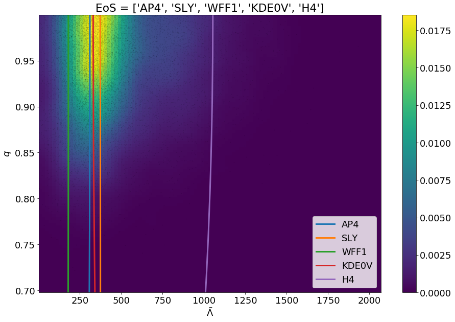
Given the choice of the equation of state models the user can plot them against the posterior distribution. The models whose curves passes-by closest to the posterior distribution (yellow-green region) have the highest Bayes-factors.

The above figure will be generated upon execution of the code snippets. The user can also supply custom equation of state models using the text file feature as discussed in the The methods section. The list of the equation of state models that the user wants to use must be passed as a python list, unless the user wants to plot just a single equation of state model, in that case just a string of the model name or the name of the file will suffice.

One can also remove the constraint on fixing the chirp mass to its mean value by passing the argument full_mc_dist=True as shown below:

modsel = ems.Model_selection(posteriorFile='samples.dat')
modsel.plot_func(['AP4', 'SLY', 'WFF1', 'KDE0V', 'H4'],
                 filename='models_with_data_full_mc_dist.png',
                 full_mc_dist=True)

This will generate a png file in the current working directory named models_with_data_full_mc_dist.png which will have the visualization.

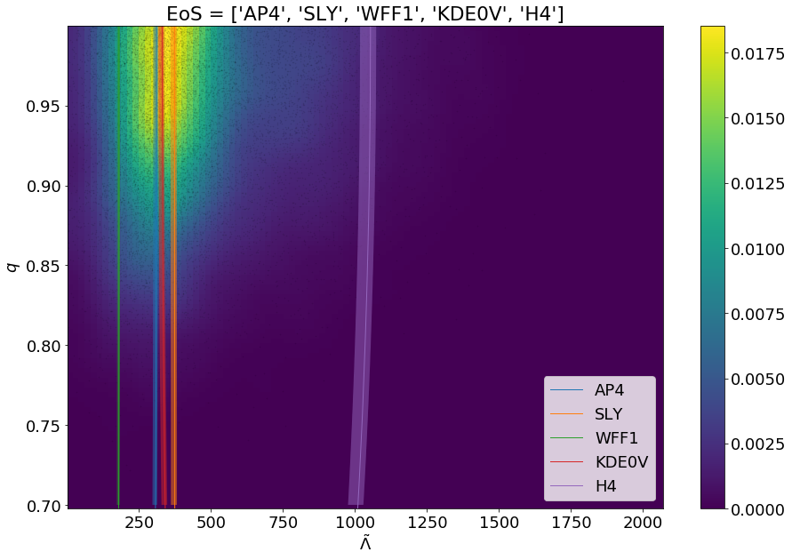
Setting the full_mc_dist boolean argument to true allows the user to get the full extent of the chirp-mass distribution in the plot.

Plotting tool for stacking:

The result of the stacking can be plotted using a plotting tool that we provide along with the package. The plotting method is a member of the Stacking class thus needs the defining of the stacking object.

from GWXtreme import eos_model_selection as ems
stackobj = ems.Stacking(['samples_1.dat', 'samples_2.dat',
                         'samples_3.dat'],
                        labels=['first event', 'second_event',
                                'third event'])
stackobj.plot_stacked_bf(eos_list=['AP4', 'SLY', 'H4'],
                         ref_eos='SLY', trials=100)

This will generate a plot in the present working directory where the results from the stacking of Bayes-factor w.r.t SLY will be plotted for the equation of states AP4, SLY, H4. The location of the plotted file can be configured using the kwarg filename.

Evidence tool for parametrized models:

The evidence for an parametrized equation of state can be computed as well.

from GWXtreme import eos_model_selection as ems
modsel = ems.Model_selection(posteriorFile='samples.dat', spectral=False)
modsel.eos_evidence([33.269,2.83,3.445,3.348])

General Comments:

Note that if the user supplies a name of the equation of state model that is not defined in LALsuite this will result in the termination of the code. Thus, an error will occur if the user does not supply the correct path to the custom data file for the equation of state model. The method will then interpret the wrongly supplied filename as an equation of state model name, and fail.

A list of all equation of state model names recognized by the version of LALsuite installed in your environment can be obtained as follows:

modsel = ems.Model_selection(posteriorFile='samples.dat')
modsel.getEoSInterp()

which will print the names of the recognized models in the standard I/O.

Contents:

• Auto Generated Documentation

Indices and tables

• Index

• Module Index

• Search Page